Examples of distributed vector usage

Vector 0: Simple vector initialization

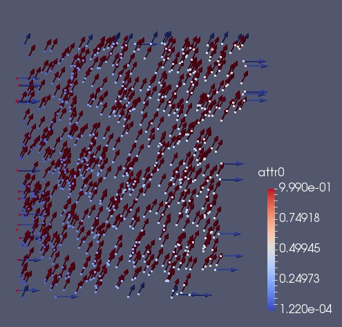
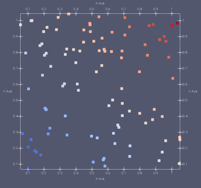
This example show several basic functionalities of the distributed vector vector_dist. The distributed vector is a set of particles in an N-dimensional space. In this example it is shown how to:

• Initialize the library
• Create a Box that defines the domain
• An array that defines the boundary conditions
• A Ghost object that will define the extension of the ghost part in physical units

The source code of the example Vector/0_simple/main.cpp. The full doxygen documentation Vector_0_simple.

See also our video lectures dedicated to this topic Video 1, Video 2

---

Example 1: Vector Ghost layer

This example shows the properties of ghost_get and ghost_put - functions that synchronize the ghosts layer for a distributed vector vector_dist.

In this example it is shown how to:

• Iterate vector_dist via getDomainIterator
• Redistribute the particles in vector_dist according to the underlying domain decomposition via map
• Synchronize the ghost layers in the standard way
• NO_POSITION, KEEP_PROPERTIES and SKIP_LABELLING options of the ghost_get function
• Propagate the data from ghost to non-ghost particles via ghost_put

The source code of the example Vector/1_ghost_get_put/main.cpp. The full doxygen documentation Vector_1_ghost_get.

---

Example 2: Cell-lists and Verlet-lists

This example shows the properties of ghost_get and ghost_put - functions that synchronize the ghosts layer for a distributed vector vector_dist.

Key points:

• How to utilize the grid iterator getGridIterator, to create a grid-like particle domain
• Two principal types of fast neighbor lists: cell-list getCellList and Verlet-list getVerlet for a distributed vector vector_dist
• CELL_MEMFAST, CELL_MEMBAL and CELL_MEMMW variations of the cell-list, with different memory requirements and computations costs
• Iterating through the neighboring particles via getNNIterator of cell-list and Verlet-list

The source code of the example Vector/1_celllist/main.cpp. The full doxygen documentation Vector_1_celllist.

---

Example 3: GPU vector

This example shows how to create a vector data-structure with vector_dist_gpu to access a vector_dist-alike data structure from GPU accelerated computing code.

Key points:

• How to convert the source code from using vector_dist to vector_dist_gpu and how it influences the memory layout of the data structure
• Oflloading particle position hostToDevicePos and particle property hostToDeviceProp data from CPU to GPU
• Lanuching a CUDA-like kernel with CUDA_LAUNCH and automatic subdivision of a computation loop into workgroups/threads via getDomainIteratorGPU or manually specifying the number of workgroups and the number of threads in a workgroup
• Passing the data-structures to a CUDA-like kernel code via toKernel
• How to use map with the option RUN_DEVICE to redistribute the particles directly on GPU, and ghost_get with RUN_DEVICE option to fill ghost particles directly on GPU
• How to detect and utilize RDMA on GPU to get the support of CUDA-aware MPI implementation to work directly with device pointers in communication subroutines

The source code of the example Vector/1_gpu_first_step/main.cpp. The full doxygen documentation Vector_1_gpu_first_step.

---

Example 4: HDF5 Save and load

This example show how to save and load a vector to/from the parallel file format HDF5.

Key points:

• How to save the position/property information of the particles vector_dist into an .hdf5 file via save
• How to load the position/property information of the particles vector_dist from an .hdf5 file via load

The source code of the example Vector/1_HDF5_save_load/main.cpp. The full doxygen documentation Vector_1_HDF5.

---

Example 5: Vector expressions

This example shows how to use vector expressions to apply mathematical operations and functions on particles. The example also shows to create a point-wise applicable function
$$A_q e^{\frac{|x_p-x_q|^2}{\sigma}}$$

where $A_q$ is the property $A$ of particle $q$, $x_p, x_q$ are positions of particles $p, q$ correspondingly.

Key points:

• Setting an alias for particle properties via getV of particle_dist to be used within an expression
• Composing expressions with scalar particle properties
• Composing expressions with vector particle properties. The expressions are 1) applied point-wise; 2) used to create a component-wise multiplication via *; 3) scalar product via pmul; 4) compute a norm norm; 5) perform square root operation sqrt
• Converting Point object into an expression getVExpr to be used with vector expressions
• Utilizing operator= and the function assign to assing singular or multiple particle properties per iteration through particles
• Constructing expressions with applyKernel_in and applyKernel_in_gen to create kernel functions called at particle locations for all the neighboring particles, e.g. as in SPH

$$\sum_{q = Neighborhood(p)} A_q D^{\beta}ker(x_p,x_q) V_q$$

The source code of the example Vector/2_expressions/main.cpp. The full doxygen documentation Vector_2_expression.

---

Example 6: Molecular Dynamics with Lennard-Jones potential (Cell-List)

This example shows a simple Lennard-Jones molecular dynamics simulation in a stable regime. The particles interact with the interaction potential
$$V(x_p,x_q) = 4( (\frac{\sigma}{r})^{12} - (\frac{\sigma}{r})^6 )$$

$A_q$ is the property $A$ of particle $q$, $x_p, x_q$ are positions of particles $p, q$ correspondingly, $\sigma$ is a free parameter, $r$ is the distance between the particles.

Key points:

• Reusing memory allocated with getCellList for the subsequent iterations via updateCellList
• Utilizing CELL_MEMBAL with getCellList to minimize memory footprint
• Performing 10000 time steps using symplectic Verlet integrator

$$\vec{v}(t_{n}+1/2) = \vec{v}_p(t_n) + \frac{1}{2} \delta t \vec{a}(t_n)$$

$$\vec{x}(t_{n}+1) = \vec{x}_p(t_n) + \delta t \vec{v}(t_n+1/2)$$

$$\vec{v}(t_{n+1}) = \vec{v}_p(t_n+1/2) + \frac{1}{2} \delta t \vec{a}(t_n+1)$$

• Producing a time-total energy 2D plot with GoogleChart

The source code of the example Vector/3_molecular_dynamic/main.cpp. The full doxygen documentation Vector_3_md_dyn.

---

Example 7: Molecular Dynamics with Lennard-Jones potential (Verlet-List) [1/3]

The physical model in the example is identical to Molecular Dynamics with Lennard-Jones potential (Cell-List). Please refer to it for futher details. Key points:

• Due to the computational cost of updating Verlet-list, r_cut + skin cutoff distance is used such that the Verlet-list has to be updated once in 10 iterations via updateVerlet
• As Verlet-lists are constructed based on local particle id's, which would be invalidated by map or ghost_get ,map is called every 10 time-step, and ghost_get is used with SKIP_LABELLING option to keep old indices every iteration

The source code of the example Vector/3_molecular_dynamic/main_vl.cpp. The full doxygen documentation Vector_3_md_vl.

---

Example 7: Molecular Dynamics with Lennard-Jones potential (Symmetric Verlet-List) [2/3]

This example is an extension to Molecular Dynamics with Lennard-Jones potential (Verlet-List). It shows how better performance can be achieved for symmetric interaction models with symmetric Verlet-list compared to the standard Verlet-list. Key points:

• Computing the interaction for particles p, q only once
• Propagate the data from potentially ghost particles q to non-ghost particles in their corresponding domains via ghost_put with the operation add_
• Changing the prefactor in the subroutine of calculating the total energy as every pair of particles is visited once (as compared to two times before)
• Updating Verlet-list once in 10 iterations via updateVerlet with 'VL_SYMMETRIC' flag

The source code of the example Vector/5_molecular_dynamic_sym/main.cpp. The full doxygen documentation Vector_5_md_vl_sym.

---

Example 7: Molecular Dynamics with Lennard-Jones potential (Symmetric CRS Verlet-List) [3/3]

This example is an extension to Molecular Dynamics with Lennard-Jones potential (Verlet-List) and Molecular Dynamics with Lennard-Jones potential (Verlet-List). It shows how better performance can be achieved for symmetric interaction models with symmetric Verlet-list compared to the standard Verlet-list. Key points:

• Computing the interaction for particles p, q only once
• Propagate the data from potentially ghost particles q to non-ghost particles in their corresponding domains via ghost_put with the operation add_
• Changing the prefactor in the subroutine of calculating the total energy as every pair of particles is visited once (as compared to two times before)
• Updating Verlet-list once in 10 iterations via updateVerlet with 'VL_SYMMETRIC' flag

The source code of the example Vector/5_molecular_dynamic_sym/main.cpp. The full doxygen documentation Vector_5_md_vl_sym.

---

Example 8: Molecular Dynamics with Lennard-Jones potential (GPU)

The physical model in the example is identical to Molecular Dynamics with Lennard-Jones potential (Cell-List) and Molecular Dynamics with Lennard-Jones potential (Verlet-List). Please refer to those for futher details. Key points:

• To get the particle index inside a CUDA-like kernel GET_PARTICLE macro is used to avoid overflow in the construction blockIdx.x * blockDim.x + threadIdx.x
• A primitive reduction function reduce_local with the operation _add_ is used to get the total energy by summing energies of all particles.

The source code of the example Vector/3_molecular_dynamic_gpu/main_vl.cpp. The full doxygen documentation Vector_3_md_dyn_gpu.

---

Example 9: Molecular Dynamics with Lennard-Jones potential (GPU optimized)

The physical model in the example is identical to Molecular Dynamics with Lennard-Jones potential (Cell-List), Molecular Dynamics with Lennard-Jones potential (Verlet-List) and is based on Molecular Dynamics with Lennard-Jones potential (GPU). Please refer to those for futher details. Key points:

• To achieve coalesced memory access on GPU and to reduce cache load the particle indices are stored in cell-list in a sorted manner, i.e. particles with neighboring indices are located in the same cell. This is achieved by assigning new particle indices and storing them temporarily in vector_dist by passing the parameter CL_GPU_REORDER to the method getCellListGPU of vector_dist. By default the method copies particle positions and no properties to the reordered vector. To copy properties as well they are passed as a template parameter <...> of the method getCellListGPU.
• The cell-list built on top of the reordered version of vector_dist uses get_sort instead of get to get a neighbor particle index when iterating with the cell-list neighborhood iterator getNNIteratorBox
• The sorted version of vector_dist have to be reordered to the original order once the processing is done via restoreOrder of vector_dist. By default the method copies particle positions and no properties to the original unordered vector. To copy properties as well they are passed as a template parameter <...> of the method restoreOrder.

The source code of the example Vector/3_molecular_dynamic_gpu_opt/main_vl.cpp. The full doxygen documentation Vector_3_md_dyn_gpu_opt.

---

Example 10: Molecular Dynamics with Lennard-Jones potential (Particle reordering)

The physical model in the example is identical to Molecular Dynamics with Lennard-Jones potential (Cell-List), Molecular Dynamics with Lennard-Jones potential (Verlet-List). The example shows how reordering the data can significantly reduce the computational running time. Key points:

• The particles inside vector_dist are reordered via reorder following a Hilbert curve of order m (here m=5) passing through the cells of $2^m \times 2^m \times 2^m$ (here, in 3D) cell-list
• It is shown that the frequency of reordering depends on the mobility of particles
• Wall clock time is measured of the function calc_force utilizing the object timer via start and stop

The source code of the example Vector/4_reorder/main_data_ord.cpp. The full doxygen documentation Vector_4_reo.

---

Example 11: Molecular Dynamics with Lennard-Jones potential (Cell-list reordering)

The physical model in the example is identical to Molecular Dynamics with Lennard-Jones potential (Cell-List), Molecular Dynamics with Lennard-Jones potential (Verlet-List). The example shows how reordering the data can significantly reduce the computational running time. Key points:

• The cell-list cells are iterated following a Hilbert curve instead of a normal left-to-right bottom-to-top cell iteration (in 2D). The function getCellList_hilb of vector_dist is used instead of getCellList
• It is shown that for static or slowly moving particles a speedup of up to 10% could be achieved

The source code of the example Vector/4_reorder/main_comp_ord.cpp. The full doxygen documentation Vector_4_comp_reo.

---

Example 12: Complex properties [1/2]

This example shows how to use complex properties in the distributed vector vector_dist

Key points:

• Creating a distributed vector with particle properties: scalar, vector float[3], Point, list of float openfpm::vector<float>, list of custom structures openfpm::vector<A> (where A is a user-defined type with no pointers), vector of vectors openfpm::vector<openfpm::vector<float>>>
• Redistribute the particles in vector_dist according to the underlying domain decomposition. Communicate only the selected particle properties via map_list (instead of communicating all map)
• Synchronize the ghost layers only for the selected particle properties ghost_get

The source code of the example Vector/4_complex_prop/main.cpp. The full doxygen documentation Vector_4_complex_prop.

---

Example 13: Complex properties [2/2]

This example shows how to use complex properties in the distributed vector vector_dist

Key points:

• Creating a distributed vector with particle properties: scalar, vector float[3], Point, list of float openfpm::vector<float>, list of custom structures openfpm::vector<A> (where A is a user-defined type with memory pointers inside), vector of vectors openfpm::vector<openfpm::vector<float>>>
• Enabling the user-defined type being serializable by vector_dist via
  • packRequest method to indicate how many byte are needed to serialize the structure
  • pack method to serialize the data-structure via methods allocate, getPointer of ExtPreAlloc and method pack of Packer
  • unpack method to deserialize the data-structure via method getPointerOffset of ExtPreAlloc and method unpack of Unpacker
  • noPointers method to inform the serialization system that the object has pointers
  • Constructing constructor, destructor and operator= to avoid memory leaks

The source code of the example Vector/4_complex_prop/main.cpp. The full doxygen documentation Vector_4_complex_prop_ser.

---

Example 14: Multiphase Cell-lists and Verlet-lists

This example is an extension to Example 2: Cell-lists and Verlet-lists and ()[]. It shows how to use multi-phase cell-lists and Verlet-list using multiple instances of vector_dist. Key points:

• All the phases have to use the same domain decomposition, which is achieved by passing the decomposition of the first phase to the constructor of vector_dist of all the other phases.
• The domains have to be iterated individually via getDomainIterator, the particles redistributed via map, the ghost layers synchronized via ghost_get for all the phases vector_dist.
• Constructing Verlet-lists for two phases (ph0, ph1) with createVerlet, where for one phase ph0 the neighoring particles of ph1 are assigned in the Verlet-list. Cell-list of ph1 has to be passed to createVerlet
• Constructing Verlet-lists for multiple phases (ph0, ph1, ph2...) with createVerletM, where for one phase ph0 the neighoring particles of ph1, ph2... are assigned in the Verlet-list. Cell-list containing all of ph1, ph2... create with createCellListM has to be passed to createVerletM
• Iterating over the neighboring particles of a multiphase Verlet-list with getNNIterator with get being substituded by getP (particle phase) and getV (particle id)
• Extending example of the symmetric interaction for multiphase cell-lists and Verlet-lists via createCellListSymM, createVerletSymM

The source code of the example Vector/4_multiphase_celllist_verlet/main.cpp. The full doxygen documentation Vector_4_mp_cl.

---

Example 16: Validation and debugging

This example shows how the flexibility of the library can be used to perform complex tasks for validation and debugging. Key points:

• To get unique global id's of the particles the function accum of vector_dist is used, which returns prefix sum of local domain sizes $j<i$ for the logical processor $i$ out of $N$ total processors
• Propagate the data from potentially ghost particles q to non-ghost particles in their corresponding domains via ghost_put with the operation merge_, that merges two openfpm::vector (ghost and non-ghost)

The source code of the example Vector/6_complex_usage/main.cpp. The full doxygen documentation Vector_6_complex_usage.

---

Example 17: Smoothed Particle Hydrodynamics (SPH) formulation on CPU [1/2]

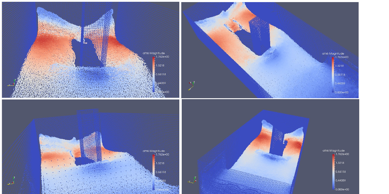
This example shows the classical SPH Dam break simulation with Load Balancing and Dynamic load balancing. The example has been adopted from DualSPHysics. Please refer to the website of DualSPHysics and to the paper of Monaghan, 1992 for more details.

Formulation

The SPH formulation used in this example code follow these equations $$\frac{d\vec{v}_a}{dt} = - \sum_{b = NN(a) } m_b \left(\frac{P_a + P_b}{\rho_a \rho_b} + \Pi_{ab} \right) \nabla_{a} W_{ab} + g$$ $$\frac{d\rho_a}{dt} = \sum_{b = NN(a) } m_b vec{v}_{ab} \cdot \nabla_{a} W_{ab}$$ $$P_a = b \left[ \left( \frac{\rho_a}{\rho_{0}} \right)^{\gamma} - 1 \right]$$

with the the viscosity term

$$\Pi_{ab} = \begin{cases} - \frac{\alpha \bar{c_{ab}} \mu_{ab} }{\bar{\rho_{ab}} } & vec{v}_{ab} \cdot r_{ab} > 0 \\ 0 & vec{v}_{ab} \cdot r_{ab} < 0 \end{cases}$$

and the constants defined as

$$b = \frac{c_{s}^{2} \rho_0}{\gamma}$$ $$c_s = \sqrt{g \cdot h_{swl}}$$

The cubic kernel $W_{ab}$ defined as

$$\begin{cases} 1.0 - \frac{3}{2} q^2 + \frac{3}{4} q^3 & 0 < q < 1 \\ (2 - q)^3 & 1 < q < 2 \\ 0 & q > 2 \end{cases}$$

its gradient $ \nabla W_{ab} $.

$$\nabla W_{ab} = \beta (x,y,z)$$

$$\beta = \begin{cases} (c_1 q + d_1 q^2) & 0 < q < 1 \\ c_2 (2 - q)^2 & 1 < q < 2 \end{cases}$$

While the particle kernel support is given by

$$H = \sqrt{3 \cdot dp}$$

where $dp$ is the particle spacing. Please refer to the work of Monaghan, 1992 for more details on the variables and constants used.

The simulation uses an additional Tensile term to avoid the tensile instability. Please refer to Monaghan, 1999 for more details on this scheme.

Time-stepping

Dynamic time stepping is calculated in accordance with Monaghan, 1992

$$\delta t = CFL \cdot min(t_f,t_{cv})$$

where

$$\delta t_f = min \sqrt{h/\vec{f_a}}$$

$$\delta t_{cv} = min \frac{h}{c_s + max \left| \frac{hv_{ab} \cdot r_{ab}}{r_{ab}^2} \right|}$$

With the governing equations are written as

$$\frac{\vec{v}_a^{n+1}}{dt} = \vec{F_a}$$

$$\frac{\rho_a^{n+1}}{dt} = D_a$$

$$\frac{\vec{r}_a^{n+1}}{dt} = \vec{v}_a$$

The Verlet time-stepping scheme Verlet, 1967 is used

$$\vec{v}_a^{n+1} = \vec{v}_a^{n-1} + 2 \delta t \vec{F_a}^{n}$$

$$\vec{r}_a^{n+1} = \delta t \vec{r}_a^n + \delta t \vec{v}_a^{n} + 0.5 \delta t^2 \vec{F_a}^n$$

$$\rho_a^{n+1} = \rho_a^{n-1} + 2 \delta t D_a^n$$

Due to the integration over a staggered time interval, the equations of density and velocity are decoupled, which may lead to divergence of the integrated values. See DualSPHysics formulation.

$$\vec{v}_a^{n+1} = \vec{v}_a^{n} + \delta t \vec{F_a}^n$$

$$\vec{r}_a^{n+1} = \vec{r}_a^{n} + \delta t \vec{v}_a^n + \frac{1}{2} \delta t^2 \vec{F_a}^n$$

$$\rho_a^{n+1} = \rho_a^n + \delta t D_a^n$$

Load Balancing

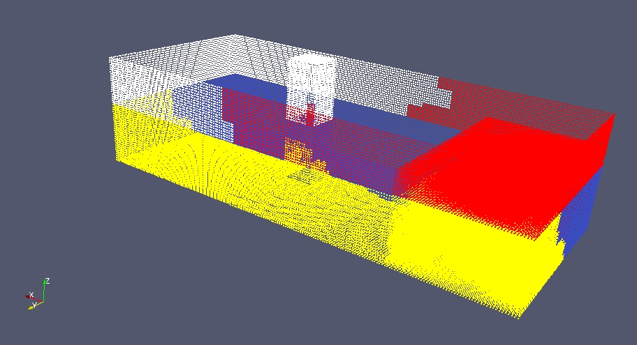
In order to reach an optimal utilization of available computational resource we distribute the particles to reach a balanced simulation. To do this we set weights for each sub-sub-domain, decompose the space and distribute the particles accordingly.

The weights are set according to:

$$w_v = 4 N_{fluid} + 3 N_{boundary}$$

where $N_{fluid}$ Is the number of fluid particles in a sub-sub-domain and $ N_{boundary} $ is the number of boundary particles.

Implicitly the communication cost is given by $ \frac{V_{ghost}}{V_{sub-sub}} t_s $, while the migration cost is given by $ v_{sub-sub} $. In general $ t_s $ is the number of ghost_get calls between two rebalance calls.

Dynamic load balancing. Theory 1
Dynamic load balancing. Theory 2
Dynamic load balancing. Practice 1
Dynamic load balancing. Practice 2

Simulation results

Simulation video 1
Simulation video 2
Simulation dynamic load balancing video 1
Simulation dynamic load balancing video 2
Simulation countour prospective 1
Simulation countour prospective 2
Simulation countour prospective 3

Key points:

• Load balancing and dynamic load balancing indicate the possibility of the system to re-adapt the domain decomposition to keep all the processor under load and reduce idle time
• Cell-list is used to iterate neighboring particles when computing derivatives
• Domain decomposition could use a user-provided cost function on sub-sub-domains later for them to be assigned to sub-domains (usually equal to the number of processors) via addComputationCosts of vector_dist
• The object DEC_GRAN(512) passed to the constructor of vector_dist is related to the Load-Balancing decomposition granularity. It indicates that the space must be decomposed in at least $ N_{subsub} $ sub-sub-domains for $ N_p $ processors

$$N_{subsub} = 512 \cdot N_p$$

• Method DrawBox of the class DrawParticles returns an iterator that can be used to create particles on a Cartesian grid with a given spacing (grid boundaries should be inside the simulation domain).
• After filling the computational cost the domain stored in vector_dist is decomposed via getDecomposition().decompose() (i.e. every sub-sub-domain is assigned to a processor) and subsequently the particles are redistributed to the corresponding processors via map.

The source code of the example Vector/7_SPH_dlb/main.cpp. The full doxygen documentation Vector_7_sph_dlb.

---

Example 17: Smoothed Particle Hydrodynamics (SPH) formulation on CPU: optimized [2/2]

The physical model in the example is identical to Example 17: Smoothed Particle Hydrodynamics (SPH) formulation on CPU.

Key points:

• Verlet-list is used instead of Cell list to iterate neighboring particles when computing derivatives. The Verlet-list is reconstructed on maximum particle displacement reaching the half skin size. Symmetric interaction reduces the computation complexity by half. Ghost particles are used to store symmetric interaction force and density increments. The increments are added to the corresponding non-ghost particles via ghost_put
• vector_dist is constructed with the option BIND_DEC_TO_GHOST. It binds the domain decomposition to be multiple of the ghost size required by the symmetric interaction
• Refine the domain decomposition instead of decomposing the domain from scratch via getDecomposition().redecompose(...) of vector_dist. Available only for ParMetis decomposition.

The source code of the example Vector/7_SPH_dlb_opt/main.cpp. The full doxygen documentation Vector_7_sph_dlb_opt.

---

Example 18: Smoothed Particle Hydrodynamics (SPH) formulation on GPU [1/3]

The physical model in the example is identical to Example 17: Smoothed Particle Hydrodynamics (SPH) formulation on CPU with the computation-heavy subroutines being executed on GPU.

Simulation results

Simulation video 1
Simulation video 2
Simulation video 3

Key points:

• Derivative approximation scheme (SPH), particle force calculation, time integration schemes (Euler, Verlet time integration) and pressure sensor readings implemented on GPU.
• A primitive reduction function reduce_local with the operation _add_ is used to get the total energy by summing energies of all particles.
• Particles exceeding the domain boundaries are removed with the GPU subroutine remove_marked<prp>, where prp is the property of vector_dist set to 1 for particles to be removed, and to 0 otherwise.

The source code of the example Vector/7_SPH_dlb_gpu/main.cu. The full doxygen documentation Vector_7_sph_dlb_gpu.

---

Example 18: Smoothed Particle Hydrodynamics (SPH) formulation on GPU: optimized [2/3]

The physical model in the example is identical to Example 18: Smoothed Particle Hydrodynamics (SPH) formulation on GPU with the computation-heavy subroutines being executed on GPU optimized for improved coalesced memory access.

Key points:

• To achieve coalesced memory access on GPU and to reduce cache load the particle indices are stored in cell-list in a sorted manner, i.e. particles with neighboring indices are located in the same cell. This is achieved by assigning new particle indices and storing them temporarily in vector_dist by passing the parameter CL_GPU_REORDER to the method getCellListGPU of vector_dist. By default the method copies particle positions and no properties to the reordered vector. To copy properties as well they are passed as a template parameter <...> of the method getCellListGPU.
• The cell-list built on top of the reordered version of vector_dist uses get_sort instead of get to get a neighbor particle index when iterating with the cell-list neighborhood iterator getNNIteratorBox
• The sorted version of vector_dist have to be reordered to the original order once the processing is done via restoreOrder of vector_dist. By default the method copies particle positions and no properties to the original unordered vector. To copy properties as well they are passed as a template parameter <...> of the method restoreOrder.

The source code of the example Vector/7_SPH_dlb_gpu_opt/main.cu. The full doxygen documentation Vector_7_sph_dlb_gpu_opt.

---

Example 18: Smoothed Particle Hydrodynamics (SPH) formulation on GPU: opetimized [3/3]

The physical model in the example is identical to Example 18: Smoothed Particle Hydrodynamics (SPH) formulation on GPU: optimized with the computation-heavy subroutines being executed on GPU optimized for improved coalesced memory access and particle force calculation performed in 2 steps.

Key points:

• The subroutine get_indexes_by_type is used to split the particles into 2 lists of fluid and boundary particle ids. Two sets of GPU kernels are devised to calculate forces and density change separately for these two types of particles.

The source code of the example Vector/7_SPH_dlb_gpu_more_opt/main.cu. The full doxygen documentation Vector_7_sph_dlb_gpu_opt.

---

Example 19: Discrete Element Method (DEM) simulation of the avalanche down the inclined plane

This example implements a Discrete Element Method (DEM) simulation using the Lorentz-force contact model.

A classical model for DEM simulations of spherical granular flows is the Silbert model, it includes a Herzian contact force and an elastic deformation of the grains. Each particles has a radius $R$, mass $m$, polar momentum $I$ and is represented by the location of its center of mass $r_{i}$.

When two particles $i$ and $j$ collide or are in contact, the elastic contact deformation is given by:

$$\delta_{ij} = 2R-r_{ij}$$

where $\vec{r_{ij}}$ is the distance vector connecting particle centers and $r_{ij} = {\lvert \vec{r}_{ij}\rvert}_2$ its module. The normal and tangential components of the relative velocity at the point of contact is given by

$$\vec{v}_{n_{ij}} = \left(\vec{v}_{ij}\cdot\vec{n}_{ij}\right)\vec{n}_{ij}$$ $$\vec{v}_{t_{ij}} = \vec{v}_{ij}-\vec{v}_{n_{ij}}-R\left(\vec{\omega}_i + \vec{\omega}_j \right)\times \vec{n}_{ij}$$

with $\vec{n_{ij}}=\vec{r_{ij}}/r_{ij}$ is the normal unit vector in direction of the distance vector, $\vec{\omega_i}$ is the angular velocity of a particle and $\vec{v_{ij}}=\vec{v_i}-\vec{v_j}$ the relative velocity between the two particles. The evolution of the elastic tangential displacement $\vec{u_{t_{ij}}}$ is integrated when two particles are in contact using:

$$\vec{u'}_{t_{ij}} = \vec{u}_{t_{ij}} + \vec{v}_{t_{ij}} \delta t$$

Where $\delta t$ is the time step size. The deformation of the contacts points is stored for each particle and for each new contact point the elastic tangential displacement is initialized with $\vec{u_{t_{ij}}} = 0$. Thus for each pair of particle interacting the normal and tangential forces become:

$$\vec{F}_{n_{ij}}=\sqrt{\frac{\delta_{ij}}{2R}}\,\,\left(k_n\delta_{ij}\vec{n}_{ij}-\gamma_n m_{\text{eff}}\vec{v}_{n_{ij}}\right) \, ,$$ $$\vec{F}_{t_{ij}}=\sqrt{\frac{\delta_{ij}}{2R}}\,\,\left(-k_t\vec{u}_{t_{ij}}-\gamma_t m_{\text{eff}}\vec{v}_{t_{ij}}\right) \, ,$$

where $k_{n,t}$ are the elastic constants in normal and tangential direction, respectively, and $\gamma_{n,t}$ the corresponding viscoelastic constants. The effective collision mass is given by $m_{\text{eff}}=\frac{m}{2}$. For each contact point in order to enforce Coulomb's law

$$\|\vec{F}_{t_{ij}}\|_2 < \|\mu\vec{F}_{n_{ij}}\|_2$$

the tangential force is bounded by the normal component force. In particular the elastic tangential displacement $\vec{u_{t_{ij}}}$ is adjusted with

$$\vec{F}_{t_{ij}} \leftarrow \vec{F}_{t_{ij}}\frac{\|\mu\vec{F}_{n_{ij}}\|_2}{\|\vec{F}_{t_{ij}}\|_2}$$

This adjustment induce a truncation of the elastic displacement. The Coulomb condition is equivalent to the case where two spheres slip against each other without inducing additional deformations. Thus the deformation is truncated using:

$$\vec{u}_{t_{ij}} = -\frac{1}{k_t}\left(\vec{F}_{t_{ij}} \sqrt{\frac{2R}{\delta_{ij}}} + \gamma_t m_{\text{eff}}\vec{v}_{t_{ij}}\right) \, .$$

Considering that each particle $i$ interact with all the particles $j$ is in touch with , the total resultant force on particle $i$ is then computed by summing the contributions of all pair particles $(i,j)$. Considering that the grains are also under the effect of the gravitational field we obtain that the total force is given by

$$\vec{F}_i^{\text{tot}}=m \vec{g} + \sum_j\left(\vec{F}_{n_{ij}}+\vec{F}_{t_{ij}}\right) \, ,$$

where $\vec{g}$ is the acceleration due to gravity. Because particles has also rotational degree of freedoms, the total torque on particle $i$ is calculated using

$$\vec{T}_i^{\text{tot}} = -R \sum_j \vec{n}_{ij}\times\vec{F}_{t_{ij}} \, .$$

$\vec{r}_i$ and angular velocities $\vec{\omega}_i$ for each particle $i$ at time step $n+1$, We integrate in time the equations using leap-frog scheme with time step given by

$$\delta t = 10^{-6}\,$$ $$\vec{v}_i^{n+1} = \vec{v}_i^n + \frac{\delta t}{m}\vec{F}_i^{\text{tot}} \, , \qquad \vec{r}_i^{n+1} = \vec{r}_i^n + \delta t \vec{v}_i^{n+1}$$ $$\vec{\omega}_i^{n+1} = \vec{\omega}_i^n + \frac{\delta t}{I_i}\vec{T}_i^{\text{tot}} \, ,$$

where $\vec{r}_i^{n},\vec{v}_i^{n},\vec{\omega}_i^{n}$ denotes respectively the position, the speed and the rotational speed of the particle $i$ at time step $n$, and $\delta t$ the time step size.

Simulation results

Simulation video 1

Key points:

• Method DrawBox of the class DrawParticles returns an iterator that can be used to create particles on a Cartesian grid with a given spacing (grid boundaries should be inside the simulation domain).
• Domain decomposition uses a quadratic cost function assigned to sub-domains as a function of the number of sub-sub-domains via addComputationCosts of vector_dist
• Refine the domain decomposition instead of decomposing the domain from scratch via getDecomposition().redecompose(...) of vector_dist. Available only for ParMetis decomposition.
• Iterating through the neighboring particles via getNNIterator of Verlet-list.
• The method updateVerlet of vector_dist is used to update an existing Verlet-list after particles have changed their positions.

The source code of the example Vector/8_DEM/main.cpp. The full doxygen documentation Vector_8_DEM.

---

Example 20: GPU CUDA interoperability

This example shows how to access and operate data arrays in GPU kernels via memory pointers obtained from distributed data-structures.

Key points:

• The concept of coalesced memory access is shown for scalar property, vector and tensor properties.
• Memory reallocation process and the concept of memory alignment is explained when extending a vector.
• The method getDeviceBuffer<...>() of a serial property vector vector returned by getPropVector of parallel vector vector_dist is used to obtain an internal device pointer for the given property.

The source code of the example Vector/9_gpu_cuda_interop/main.cu. The full doxygen documentation 9_gpu_cuda_interop.

---